Understanding Perlin Noise
Technical Writeup Posted on 09 August 2014 by Flafla2
The objective of this article is to present an easy-to-understand analysis of Ken Perlin's Improved Perlin Noise. The code in this article is written in C# and is free to use. If you would prefer to just look at the final result, you can view the final source here.
Perlin Noise is an extremely powerful algorithm that is used often in procedural content generation. It is especially useful for games and other visual media such as movies. The man who created it, Ken Perlin, won an academy award for the original implementation. In this article I will be exploring his Improved Perlin Noise, published in 2002. In game development, Perlin Noise can be used for any sort of wave-like, undulating material or texture. For example, it could be used for procedural terrain (Minecraft-like terrain can be created with Perlin Noise, for example), fire effects, water, and clouds. These effects mostly represent Perlin noise in the 2nd and 3rd dimensions, but it can be extended into the 4th dimension rather trivially. Additionally Perlin Noise can be used in only 1 dimension for purposes such as side-scrolling terrain(such as in Terraria or Starbound) or to create the illusion of handwritten lines.
Also, if you extend Perlin Noise into an additional dimension and consider the extra dimension as time, you can animate it. For example, 2D Perlin Noise can be interpreted as Terrain, but 3D noise can similarly be interpreted as undulating waves in an ocean scene. Below are some pictures of Noise in different dimensions and some of their uses at runtime:
| Noise Dimension | Raw Noise (Grayscale) | Use Case |
|---|---|---|
| 1 | 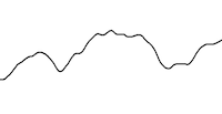 |
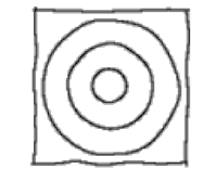 Using noise as an offset to create handwritten lines. |
| 2 |  |
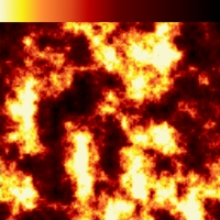 By applying a simple gradient, a procedural fire texture can be created. |
| 3 | 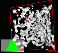 |
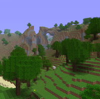 Perhaps the quintessential use of Perlin noise today, terrain can be created with caves and caverns using a modified Perlin Noise implementation. |
So as you can see, Perlin Noise has an application to many naturally-occurring phenomenon. Now let's look into the mathematics and logic of the Perlin Noise Algorithm.
Logical Overview
NOTE: I would like to preface this section by mentioning that a lot of it is taken from this wonderful article by Matt Zucker. However, that article is based on the original Perlin Noise algorithm written in the early 1980s. In this post I will be using the Improved Perlin Noise Algorithm written in 2002. Thus, there are some key differences between my version and Zucker's.
Let's start off with the basic Perlin Noise function:
public double perlin(double x, double y, double z);So we have an x, y and z coordinate as input, and as the output we get a double between 0.0 and 1.0. So what do we do with this input? First, we divide the x, y, and z coordinates into unit cubes. In other words, find [x,y,z] % 1.0 to find the coordinate's location within the cube. Below is a representation of this concept in 2 dimensions:
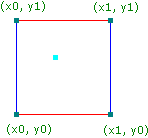
Figure 1: The blue dot here represents an input coordinate, and the other 4 points are the surrounding integral unit coordinates. (Source)
On each of the 4 unit coordinates (8 in 3D), we generate what's called a pseudorandom gradient vector. This gradient vector defines a positive direction (in the direction that it points to) and of course a negative direction (in the direction opposite that it points to). Pseudorandom means that, for any set of integers inputted into the gradient vector equation, the same result will always come out. Thus, it seems random, but it isn't in reality. Additionally this means that each integral coordinate has its "own" gradient that will never change if the gradient function doesn't change.
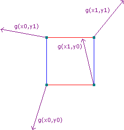
Figure 2: Based on the above image, here are some example gradient vectors. (Source)
The image above is not completely accurate, however. In Ken Perlin's Improved Noise, which we are using in this article, these gradients aren't completely random. Instead, they are picked from the vectors of the point in the center of a cube to the edges of the cube:
(1,1,0),(-1,1,0),(1,-1,0),(-1,-1,0),
(1,0,1),(-1,0,1),(1,0,-1),(-1,0,-1),
(0,1,1),(0,-1,1),(0,1,-1),(0,-1,-1)
The reasoning behind these specific gradient vectors is described in Ken Perlin's SIGGRAPH 2002 paper: Improving Noise. NOTE: Many other articles about Perlin Noise refer to the original Perlin Noise algorithm, which does not use these vectors. For example, Figure 2 represents the original algorithm because its source was written before the improved algorithm was released. However, the basic idea is the same.
Next, we need to calculate the 4 vectors (8 in 3D) from the given point to the 8 surrounding points on the grid. An example case of this in 2D is shown below.
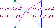
Figure 3: Example distance vectors. (Source)
Next, we take the dot product between the two vectors (the gradient vector and the distance vector). This gives us our final influence values:
grad.x * dist.x + grad.y * dist.y + grad.z * dist.z
This works because the dot product of 2 vectors is equal to the cosine of the angle between the two vectors, multiplied by the magnitude of those vectors:
dot(vec1,vec2) = cos(angle(vec1,vec2)) * vec1.length * vec2.length
In other words, if the 2 vectors are pointing in the same direction the dot product would equal:
1 * vec1.length * vec2.length
..and if the two vectors are pointing in opposite directions the dot product would equal:
-1 * vec1.length * vec2.length
If the two vectors are perpendicular, the dot product is 0.
Thus, the result of the dot product would be positive when it is in the direction of the gradient, and negative when it is in the opposite. This is how the gradient vectors define positive and negative directions. Here is a graphic representing these positive/negative influences:
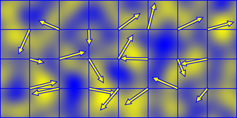
Figure 4: A representation of these influences in 2D noise. (Source)
So now all we need to do is interpolate between these 4 values so that we get a sort of weighted average in between the 4 grid points (8 in 3D). The solution to this is easy: average the averages like so (this example is in 2D):
// Below are 4 influence values in the arrangement:
// [g1] | [g2]
// -----------
// [g3] | [g4]
int g1, g2, g3, g4;
int u, v;   // These coordinates are the location of the input coordinate in its unit square.
            // For example a value of (0.5,0.5) is in the exact center of its unit square.

int x1 = lerp(g1,g2,u);
int x2 = lerp(g3,h4,u);

int average = lerp(x1,x2,v);
There is one final piece to this puzzle: with the above weighted average, the final result would look bad because linear interpolation, while computationally cheap, looks unnatural. We need a smoother transition between gradients. So, we use a fade function, also called an ease curve:
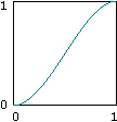
Figure 5: This is an ease curve. (Source)
This ease curve is applied to the u and v values in the above code example. This makes changes more gradual as one approaches integral coordinates. The fade function for the improved perlin noise implementation is this:
6t5-15t4+10t3
Logically, that's it! We now have all of the components needed to generate Perlin Noise. Now let's jump into some code.
Code Implementation
Once again, this code is written in C#. The code is a slightly modified version of Ken Perlin's Java Implementation. It was modified for additional clarity and deobfuscation, as well as adding the ability to repeat (tile) noise. The code is of course entirely free to use (considering I didn't really write it in the first place - Ken Perlin did!).
Setting Up
The first thing we need to do is set up our permutation table, or the p[] array for short. This is simply a length 256 array of random values from 0 - 255 inclusive. We also repeat this array (for a total size of 512) to avoid buffer overflow later on:
private static readonly int[] permutation = { 151,160,137,91,90,15,                 // Hash lookup table as defined by Ken Perlin.  This is a randomly
    131,13,201,95,96,53,194,233,7,225,140,36,103,30,69,142,8,99,37,240,21,10,23,    // arranged array of all numbers from 0-255 inclusive.
    190, 6,148,247,120,234,75,0,26,197,62,94,252,219,203,117,35,11,32,57,177,33,
    88,237,149,56,87,174,20,125,136,171,168, 68,175,74,165,71,134,139,48,27,166,
    77,146,158,231,83,111,229,122,60,211,133,230,220,105,92,41,55,46,245,40,244,
    102,143,54, 65,25,63,161, 1,216,80,73,209,76,132,187,208, 89,18,169,200,196,
    135,130,116,188,159,86,164,100,109,198,173,186, 3,64,52,217,226,250,124,123,
    5,202,38,147,118,126,255,82,85,212,207,206,59,227,47,16,58,17,182,189,28,42,
    223,183,170,213,119,248,152, 2,44,154,163, 70,221,153,101,155,167, 43,172,9,
    129,22,39,253, 19,98,108,110,79,113,224,232,178,185, 112,104,218,246,97,228,
    251,34,242,193,238,210,144,12,191,179,162,241, 81,51,145,235,249,14,239,107,
    49,192,214, 31,181,199,106,157,184, 84,204,176,115,121,50,45,127, 4,150,254,
    138,236,205,93,222,114,67,29,24,72,243,141,128,195,78,66,215,61,156,180
};

private static readonly int[] p;                                                    // Doubled permutation to avoid overflow

static Perlin() {
    p = new int[512];
    for(int x=0;x<512;x++) {
        p[x] = permutation[x%256];
    }
}
The p[] array is used in a hash function that will determine what gradient vector to use later on. The specifics of this will be explained later.
Next, we begin our perlin noise function:
public double perlin(double x, double y, double z) {
    if(repeat > 0) {                                    // If we have any repeat on, change the coordinates to their "local" repetitions
        x = x%repeat;
        y = y%repeat;
        z = z%repeat;
    }

    int xi = (int)x & 255;                              // Calculate the "unit cube" that the point asked will be located in
    int yi = (int)y & 255;                              // The left bound is ( |_x_|,|_y_|,|_z_| ) and the right bound is that
    int zi = (int)z & 255;                              // plus 1.  Next we calculate the location (from 0.0 to 1.0) in that cube.
    double xf = x-(int)x;
    double yf = y-(int)y;
    double zf = z-(int)z;

    // ...
}
This code is pretty self explanatory. First, we use the modulo (remainder) operator to have our input coordinates overflow if they are over the repeat variable. Next, we create variables xi, yi, zi. These represent the unit cube that our coordinate is in. We also bind our coordinates to the range [0,255] inclusive so that we won't run into overflow errors later on when we access the p[] array. This also has an unfortunate side effect: Perlin noise always repeats every 256 coordinates. This isn't a problem though because decimal coordinates are possible with perlin noise. Finally we find the location of our coordinate inside its unit cube. This is essentially n = n % 1.0 where n is a coordinate.
The Fade Function
Now we need to define our fade function, described above (Figure 5). As mentioned earlier, this is the Perlin Noise fade function:
6t5-15t4+10t3
In code, it is defined like this:
public static double fade(double t) {
                                                        // Fade function as defined by Ken Perlin.  This eases coordinate values
                                                        // so that they will ease towards integral values.  This ends up smoothing
                                                        // the final output.
    return t * t * t * (t * (t * 6 - 15) + 10);         // 6t^5 - 15t^4 + 10t^3
}

public double perlin(double x, double y, double z) {
    // ...

    double u = fade(xf);
    double v = fade(yf);
    double w = fade(zf);

    // ...
}
The u / v / w values will be used later with interpolation.
The Hash Function
The Perlin Noise hash function is used to get a unique value for every coordinate input. A hash function, as defined by wikipedia, is:
…any function that can be used to map data of arbitrary size to data of fixed size, with slight differences in input data producing very big differences in output data.
This is the hash function that Perlin Noise uses. It uses the p[] table that we created earlier:
public double perlin(double x, double y, double z) {
    // ...

    int aaa, aba, aab, abb, baa, bba, bab, bbb;
    aaa = p[p[p[    xi ]+    yi ]+    zi ];
    aba = p[p[p[    xi ]+inc(yi)]+    zi ];
    aab = p[p[p[    xi ]+    yi ]+inc(zi)];
    abb = p[p[p[    xi ]+inc(yi)]+inc(zi)];
    baa = p[p[p[inc(xi)]+    yi ]+    zi ];
    bba = p[p[p[inc(xi)]+inc(yi)]+    zi ];
    bab = p[p[p[inc(xi)]+    yi ]+inc(zi)];
    bbb = p[p[p[inc(xi)]+inc(yi)]+inc(zi)];

    // ...
}

public int inc(int num) {
    num++;
    if (repeat > 0) num %= repeat;

    return num;
}
The above hash function hashes all 8 unit cube coordinates surrounding the input coordinate. inc() is simply used to increment the numbers and make sure that the noise still repeats. If you didn’t care about the ability to repeat, inc(xi) can be replaced by xi+1. The result of this hash function is a value between 0 and 255 (inclusive) because of our p[] array.
The Gradient Function
I have always thought that Ken Perlin's original grad() function is needlessly complicated and confusing. Remember, the goal of grad() is to calculate the dot product of a randomly selected gradient vector and the 8 location vectors. Ken Perlin used some fancy bit-flipping code to accomplish this:
public static double grad(int hash, double x, double y, double z) {
    int h = hash & 15;                                    // Take the hashed value and take the first 4 bits of it (15 == 0b1111)
    double u = h < 8 /* 0b1000 */ ? x : y;                // If the most significant bit (MSB) of the hash is 0 then set u = x.  Otherwise y.

    double v;                                             // In Ken Perlin's original implementation this was another conditional operator (?:).  I
                                                          // expanded it for readability.

    if(h < 4 /* 0b0100 */)                                // If the first and second significant bits are 0 set v = y
        v = y;
    else if(h == 12 /* 0b1100 */ || h == 14 /* 0b1110*/)  // If the first and second significant bits are 1 set v = x
        v = x;
    else                                                  // If the first and second significant bits are not equal (0/1, 1/0) set v = z
        v = z;

    return ((h&1) == 0 ? u : -u)+((h&2) == 0 ? v : -v); // Use the last 2 bits to decide if u and v are positive or negative.  Then return their addition.
}
Below is an alternate way of writing the above code in a much more easy-to-understand way (and actually faster in many languages):
// Source: http://riven8192.blogspot.com/2010/08/calculate-perlinnoise-twice-as-fast.html
public static double grad(int hash, double x, double y, double z)
{
    switch(hash & 0xF)
    {
        case 0x0: return  x + y;
        case 0x1: return -x + y;
        case 0x2: return  x - y;
        case 0x3: return -x - y;
        case 0x4: return  x + z;
        case 0x5: return -x + z;
        case 0x6: return  x - z;
        case 0x7: return -x - z;
        case 0x8: return  y + z;
        case 0x9: return -y + z;
        case 0xA: return  y - z;
        case 0xB: return -y - z;
        case 0xC: return  y + x;
        case 0xD: return -y + z;
        case 0xE: return  y - x;
        case 0xF: return -y - z;
        default: return 0; // never happens
    }
}
The source of the above code can be found here. In any case, both versions do the same thing. They pick a random vector from the following 12 vectors:
(1,1,0),(-1,1,0),(1,-1,0),(-1,-1,0),
(1,0,1),(-1,0,1),(1,0,-1),(-1,0,-1),
(0,1,1),(0,-1,1),(0,1,-1),(0,-1,-1)
This is determined by the last 4 bits of the hash function value (the first parameter of grad()). The other 3 parameters represent the location vector (that will be used for the dot product).
Putting it all Together
Now, we take all of these functions, use them for all 8 surrounding unit cube coordinates, and interpolate them together:
public double perlin(double x, double y, double z) {
    // ...

    double x1, x2, y1, y2;
    x1 = lerp(    grad (aaa, xf  , yf  , zf),           // The gradient function calculates the dot product between a pseudorandom
                grad (baa, xf-1, yf  , zf),             // gradient vector and the vector from the input coordinate to the 8
                u);                                     // surrounding points in its unit cube.
    x2 = lerp(    grad (aba, xf  , yf-1, zf),           // This is all then lerped together as a sort of weighted average based on the faded (u,v,w)
                grad (bba, xf-1, yf-1, zf),             // values we made earlier.
                  u);
    y1 = lerp(x1, x2, v);

    x1 = lerp(    grad (aab, xf  , yf  , zf-1),
                grad (bab, xf-1, yf  , zf-1),
                u);
    x2 = lerp(    grad (abb, xf  , yf-1, zf-1),
                  grad (bbb, xf-1, yf-1, zf-1),
                  u);
    y2 = lerp (x1, x2, v);

    return (lerp (y1, y2, w)+1)/2;                      // For convenience we bind the result to 0 - 1 (theoretical min/max before is [-1, 1])
}

// Linear Interpolate
public static double lerp(double a, double b, double x) {
    return a + x * (b - a);
}
Working with Octaves
One final thing I would like to discuss is how to process perlin noise to look more natural. Even though perlin noise does provide a certain degree of natural behavior, it doesn’t fully express the irregularities that one might expect in nature. For example, a terrain has large, sweeping features such as mountains, smaller features such as hills and depressions, even smaller ones such as boulders and large rocks, and very small ones like pebbles and minute differences in the terrain. The solution to this is simple: you take multiple noise functions with varying frequencies and amplitudes, and add them together. Of course, frequency refers to the period at which data is sampled, and amplitude refers to the range at which the result can be in.
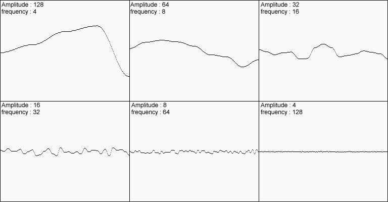
Figure 6: 6 Example noise results with differing frequencies and amplitudes. (Source)
Add all of these results together, and you get this:
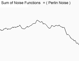
Figure 7: The addition of the 7 above results. (Source)
Obviously this result is much more convincing. The above 6 sets of noise are called different octaves of noise. Each successive octave has less and less influence on the final result. Of course, with each octave there is a linear increase in code execution time, so you should try not to use more than just a few octaves at runtime (for example, with a procedural fire effect running at 60fps). However, octaves are great when preprocessing data (such as generating terrain).
But how much influence should each successive octave have, quantitatively? This question is answered by another value called persistence. Hugo Elias defines Persistence as follows:
frequency = 2i
amplitude = persistencei
Where i is the octave in question. In code, the implementation is simple:
public double OctavePerlin(double x, double y, double z, int octaves, double persistence) {
    double total = 0;
    double frequency = 1;
    double amplitude = 1;
    double maxValue = 0;  // Used for normalizing result to 0.0 - 1.0
    for(int i=0;i<octaves;i++) {
        total += perlin(x * frequency, y * frequency, z * frequency) * amplitude;

        maxValue += amplitude;

        amplitude *= persistence;
        frequency *= 2;
    }

    return total/maxValue;
}
Conclusion
Finally, that's it! We can now make noise. Once again, you can find the full source code here. If you have any questions, please ask in the comments section below.
References
Here are some references that you can check out if you are interested:
- Ken Perlin's "Official" Improved Perlin Noise - This is the original algorithm as written by Ken Perlin.
- "The Perlin Noise Math FAQ" - This is excellent as a theoretical reference about the algorithm. Keep in mind however that it uses the original Perlin Noise algorithm from the 80s, not the one that I used in this tutorial.
- Hugo Elias' article - One of the most popular Perlin Noise articles. This is a good reference about octaves, persistence, and some uses of perlin noise in the real world. However, this is not true perlin noise! Hugo's algorithm is not based on gradients like Perlin Noise is. Instead it is what's known as value noise, which is essentially blurred white noise. Do not confuse yourself!
- "How to use Perlin Noise in Your Games" - Devmag - A cool article about some potential uses of Perlin Noise. A very interesting read, but once again this is NOT true perlin noise! Devmag uses value noise in that article.
- GPU Gems - "Implementing Improved Perlin Noise" - This article taps into the awesome power of the GPU to render stunning ocean scenes in realtime using Perlin Noise. Shaders are cool!
Thank you for reading!
Updates
8/9/14 - I have updated the article to include a better explanation about dot products, and I fixed some typos in the article. Huge thanks to all of the advice given to me by reddit /r/programming, /r/gamedev, and /r/Unity3D.
